

Directives
Dec 11, 2025
Signal Architecture
Constrained vs. Unconstrained Logic
by CelestialEye | Quantitative Systems Engineer
Signal Architecture: Constrained vs. Unconstrained
In Traditional Finance (TradFi), signal constraints are structural. Unconstrained implies absolute selection (e.g., top decile momentum), while Constrained implies sector neutrality to isolate alpha from beta factors.
The Crypto Market Structure Problem: In digital assets, cross-sectional correlations approach 1.0. Sector neutrality is ineffective because idiosyncratic risk is overwhelmed by systemic beta. Therefore, we must reframe the constraint framework from Sector Allocation to Convexity Profile.
Stability: Variance minimization.
Convexity: Maximization of positive skew (asymmetric upside).
Unconstrained Signals: Logic and Mechanics
The mandate of an unconstrained signal in crypto is pure convexity extraction. The system prioritizes exposure to the generative driver (e.g., trend) over protection of capital during lower-volatility periods.
Operational Logic
Regime Primacy: Execution is dictated solely by signal validity. If the macro condition (e.g., positive momentum) exists, the system forces exposure.
Path Independence: Recent trade outcomes are irrelevant. If a position is stopped out but the signal remains valid on the subsequent bar, the system immediately re-enters.
The Drawdown Mechanics: During mean reversion or trend exhaustion, this logic induces "whipsaw" losses. The system will incur serial stop-outs until the signal invalidates. This results in a low win rate and high psychological friction for manual execution.
Statistical Profile: Edge vs. Risk
This methodology optimizes for Positive Skewness and High Kurtosis (fat tails).
The Edge (Why it works): High-velocity upside repricing events often occur immediately following liquidity flushes (stop hunts).
A risk-averse system stays flat after a stop-out, missing the subsequent expansion.
The Unconstrained System captures the entire right-tail event because it systematically re-engages risk as long as the regime holds.
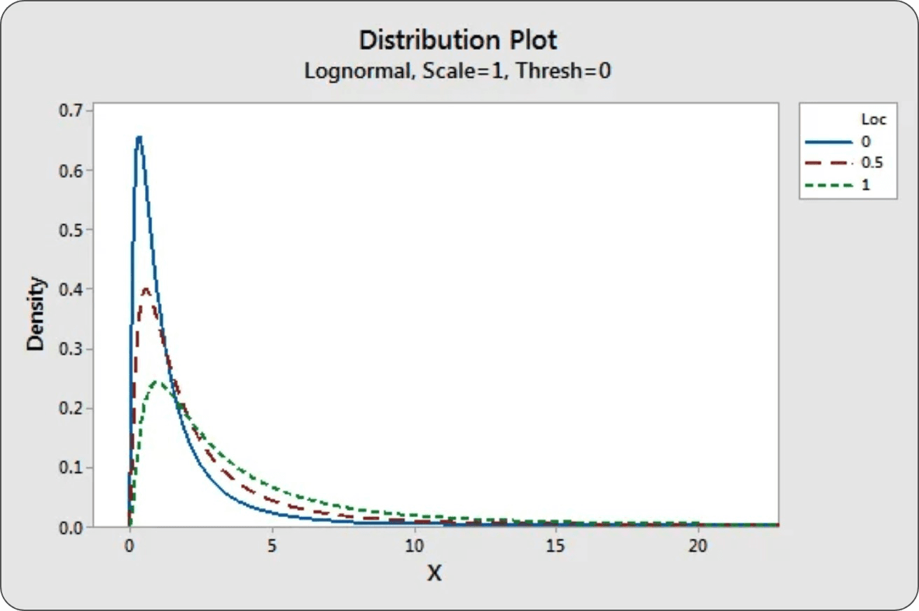
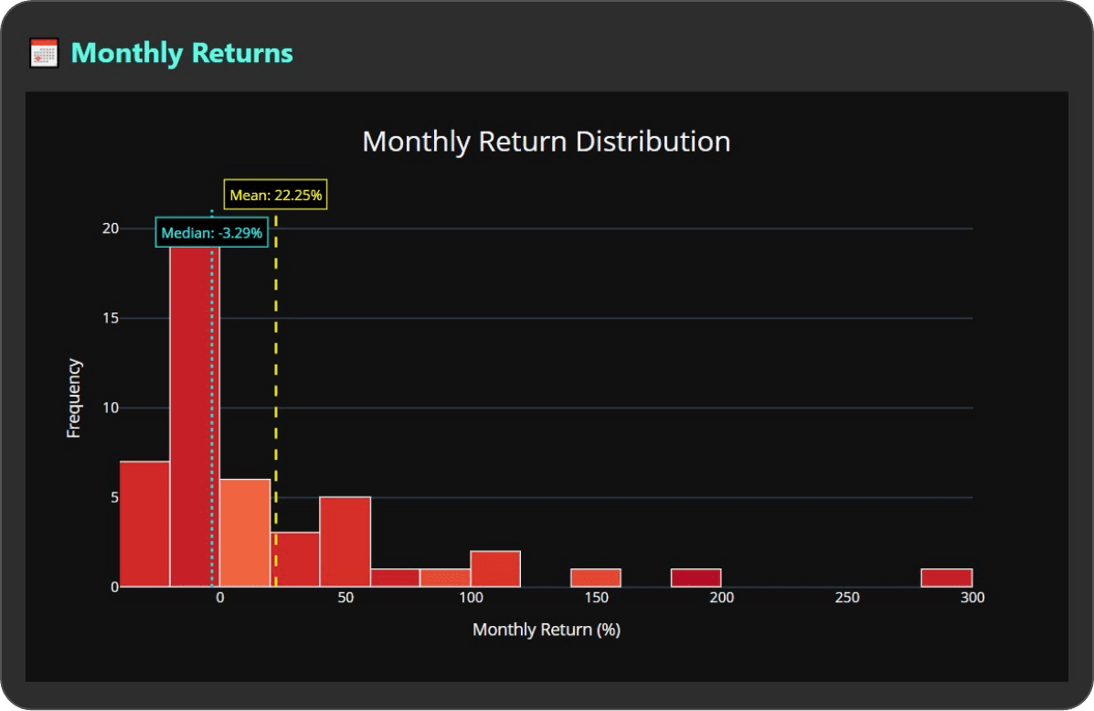
The Payoff Distribution: The return profile approximates a Log-Normal Distribution:
Left Tail (Risk): Strictly truncated at the Stop Loss level (capped downside).
Mode: Slightly negative (frequent small losses/cost of business).
Right Tail (Reward): Uncapped. The capture of extreme outliers drives the portfolio's total expectancy.
This prioritizes Expectancy (Total PnL) over Accuracy (Win Rate).
This would roughly look like this:
Constrained Signals: Stability & Variance Minimization
While unconstrained signals maximize geometric growth via volatility capture, Constrained Signals prioritize risk-adjusted returns (Sharpe) and psychological sustainability.
Operational Mechanics:
State-Transition Entry: Execution occurs only at the inception of a specific regime (e.g., Trend Flip: Neutral → Short).
Suppressed Re-entry: If a position is stopped out while the macro condition remains valid, the system remains flat. No new risk is deployed until the signal fully resets.
The Edge vs. Risk:
Edge: Prevents capital erosion during "chop" or low-quality trend extensions. Optimizes for volatility-targeted mandates.
Risk: Opportunity cost. The system will miss late-stage trend acceleration if the initial entry was stopped out.
Nomenclature Mapping
To align crypto-native slang with quantitative structure:
Unconstrained = Continuous Exposure / "Always-In"
Constrained = State-Transition Entry / "One-Shot"
BMD Strategy Implementation
The BMD model strictly utilizes a Constrained Architecture.
Execution Logic:
Entry: Triggered only on a fresh trend signal (e.g., Short generation).
Invalidation: If the trade stops out, the specific signal instance is "burned."
Reset Condition: To re-engage the short side, the asset must cycle through a non-short state (Neutral or Long). Only a subsequent transition back to Short triggers a new entry.
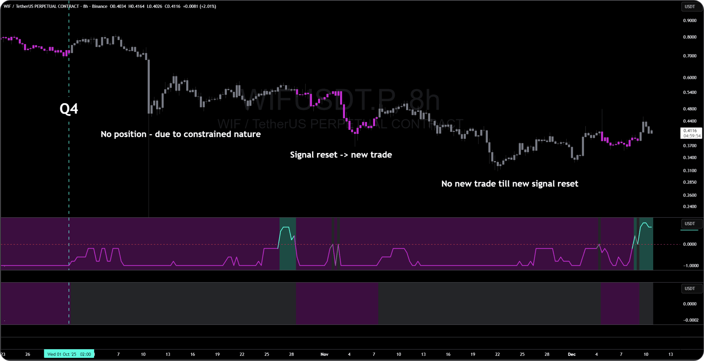
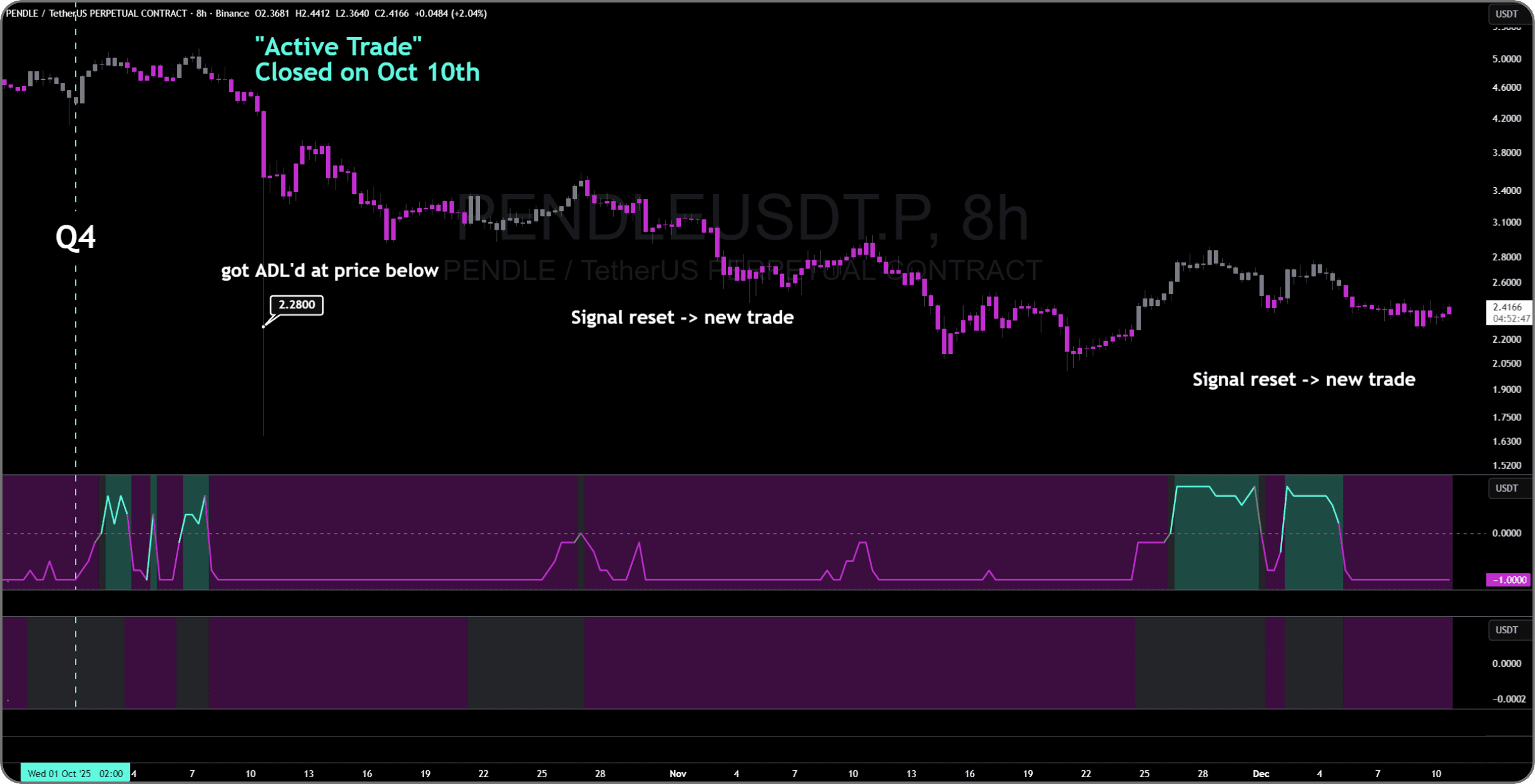
Regime Continuity (Q4 Case Study):
This logic applies strictly to the token change instances.
Stale Signals: If an asset enters a new quarter (Q4) while already in a mature negative trend, no allocation is assigned. The system does not chase existing exposure.
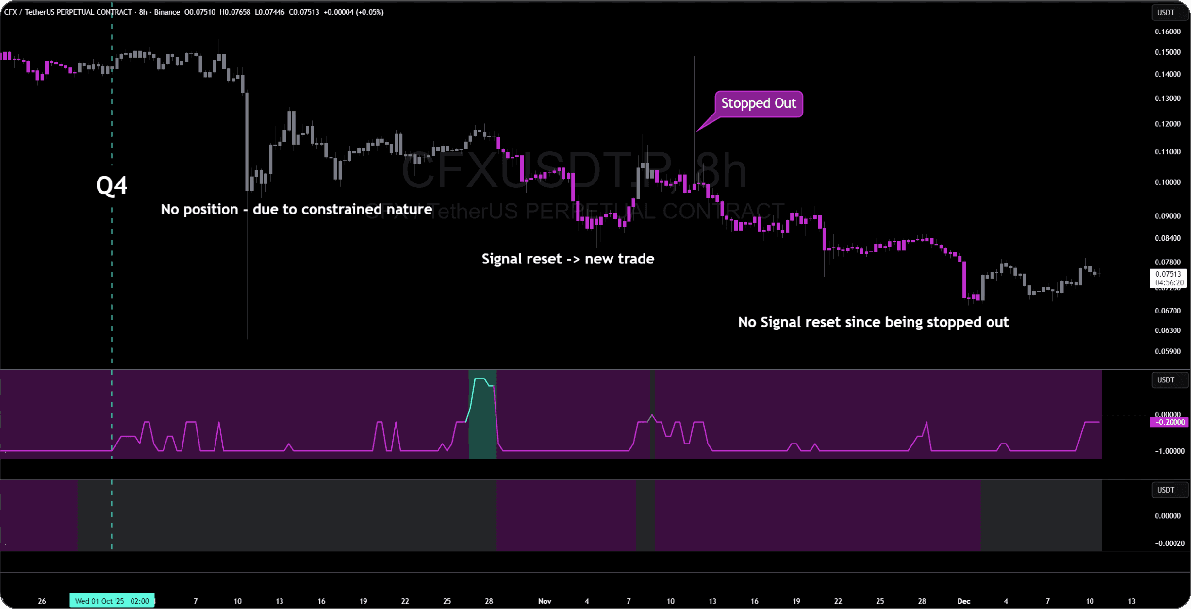
Specifics: Both WIF and CFX entered Q4 carrying existing short signals.
Result: The system remained flat on these assets despite the negative trend.
Reset: Allocation eligibility was restored only after the regime reset occurred on October 26.
Chart Anatomy:
Pane 1 (Regime): Underlying Trend Signal.
Pane 2 (Execution): Derived Trade Output (Constrained logic; raw signal before ADL/Stop filters).
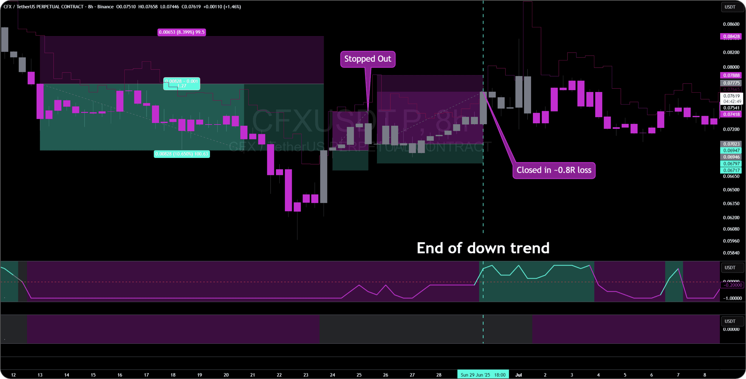
WIF:
CFX:
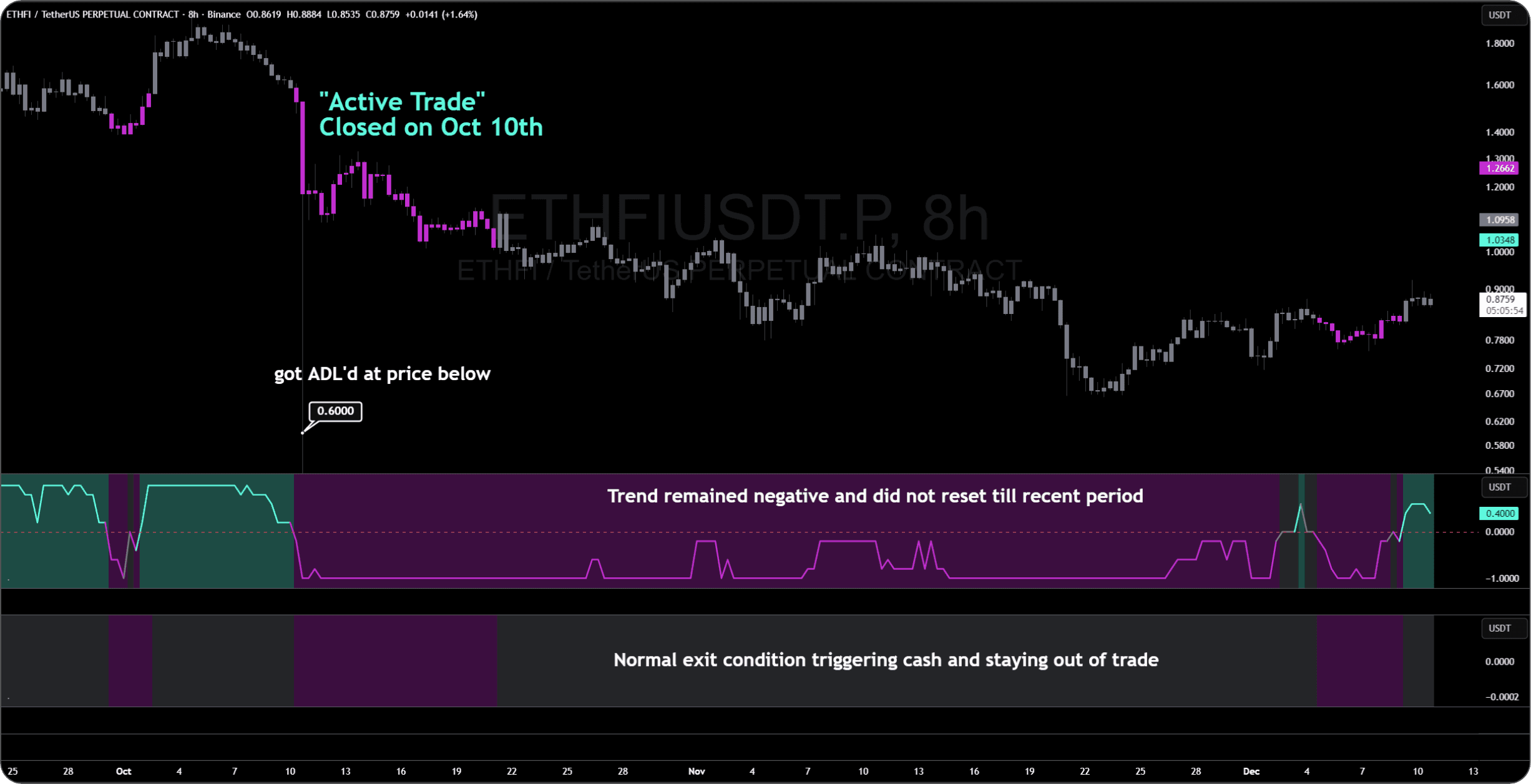
While ETHFI resets its state on Dec 2nd after a successful trade:
PENDLE:
Constrained vs. Unconstrained Signal Architecture
The primary distinction lies in the convexity profile. We privilege the constrained signal because the unconstrained variant structurally suffers from a suppressed hit rate.
In the pursuit of maximizing convexity, unconstrained systems naturally incur frequent losses, usually to close between -0.5R to -1R. This skewed distribution is a feature, not a bug, of convexity-maxing strategies across all asset classes.
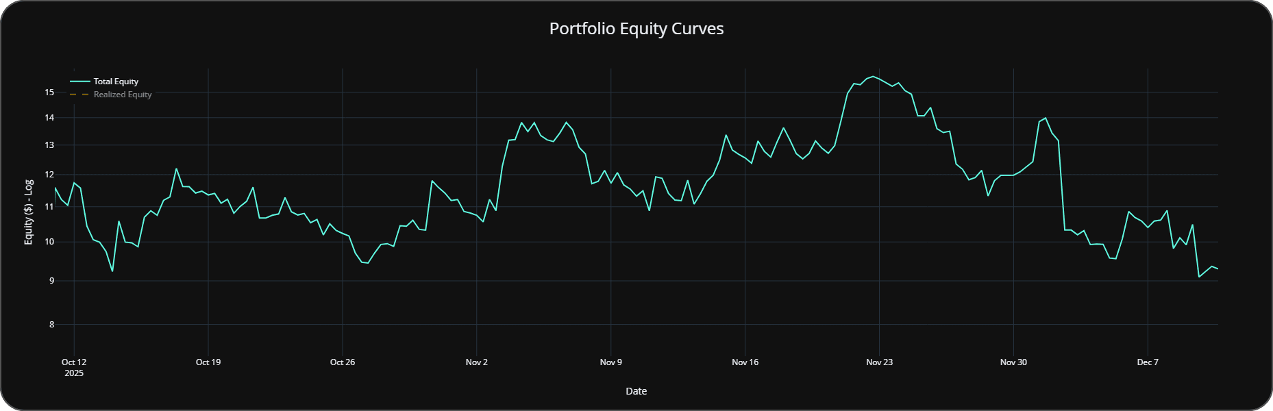
Portfolio Integration & Risk Profile
Both signal topologies are functional, but their utility depends entirely on the broader portfolio construction.
For the active Dual Portfolio (Trend Long/Short), the constrained signal offers superior risk-adjusted returns.
Unconstrained: Maximizes terminal equity only when utilized within a highly factor-diversified book. Standalone, it is psychologically and mathematically difficult to hold, exhibiting drawdowns nearly 2x deeper than the constrained model.
Performance: Since October 10th, the unconstrained system has underperformed the standard BMD in absolute terms, carrying higher realized volatility without commensurate upside capture.
Exit Mechanics: The Optimization Dilemma
A common inquiry regards the precise timing of liquidation events. It is vital to understand that there is no singular optimal exit; there is only a structural trade-off between volatility tolerance and profit protection.
We optimize along a spectrum:
Volatility Wrapping: Utilizing wide bands to accommodate standard variance.
Trend Sensitivity: utilizing short-term lookbacks for rapid exposure reduction.
The Duration/Volatility Trade-off
Trend following inherently requires absorbing volatility to capture the fat tail.
Tight Criteria: Optimizes for velocity but dramatically increases whipsaw risk. As shown in the Pendle example below, a tight volatility band forces premature exits during noise-based mean reversion (highlighted in white).
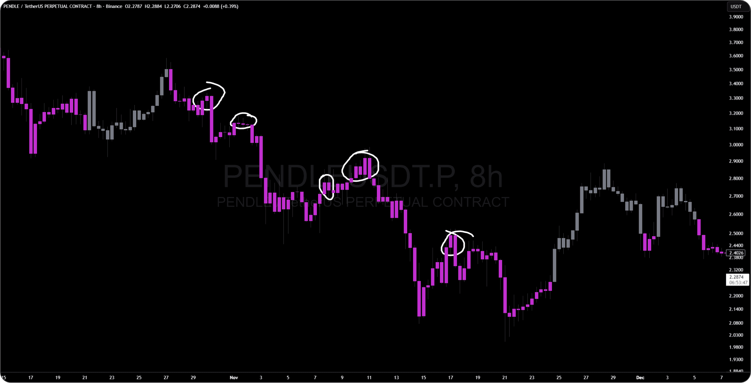
Loose Criteria: Accommodates variance but risks significant open profit give-back. A loose structure may result in exiting at the local top of a corrective bounce (gray zone), surrendering returns.
Ensemble Exit Methodology
To resolve this parameterization paradox, we reject single-trigger reliance.
The current execution model employs an ensemble of 17 distinct signals. Rather than risking the failure of a single indicator, the system utilizes a voting mechanism. This aggregates inputs to establish a confidence level, ensuring exits occur only when the probability of structural trend decay outweighs the cost of holding.
Token Selection Architecture
The strategic rationale behind the Token Selection Filter is rigorous: we aim to systematically exploit the structural downside skew inherent in mid-cap assets.
Mid-caps historically demonstrate higher velocity downside repricing compared to majors, providing a cleaner convexity profile for short strategies.
The Liquidity Constraint
However, execution reality dictates strategy. The primary friction point is available liquidity on Hyperliquid (HL), specifically following the Oct 10th deleveraging event which compressed global Open Interest (OI) from 14B → 6B.
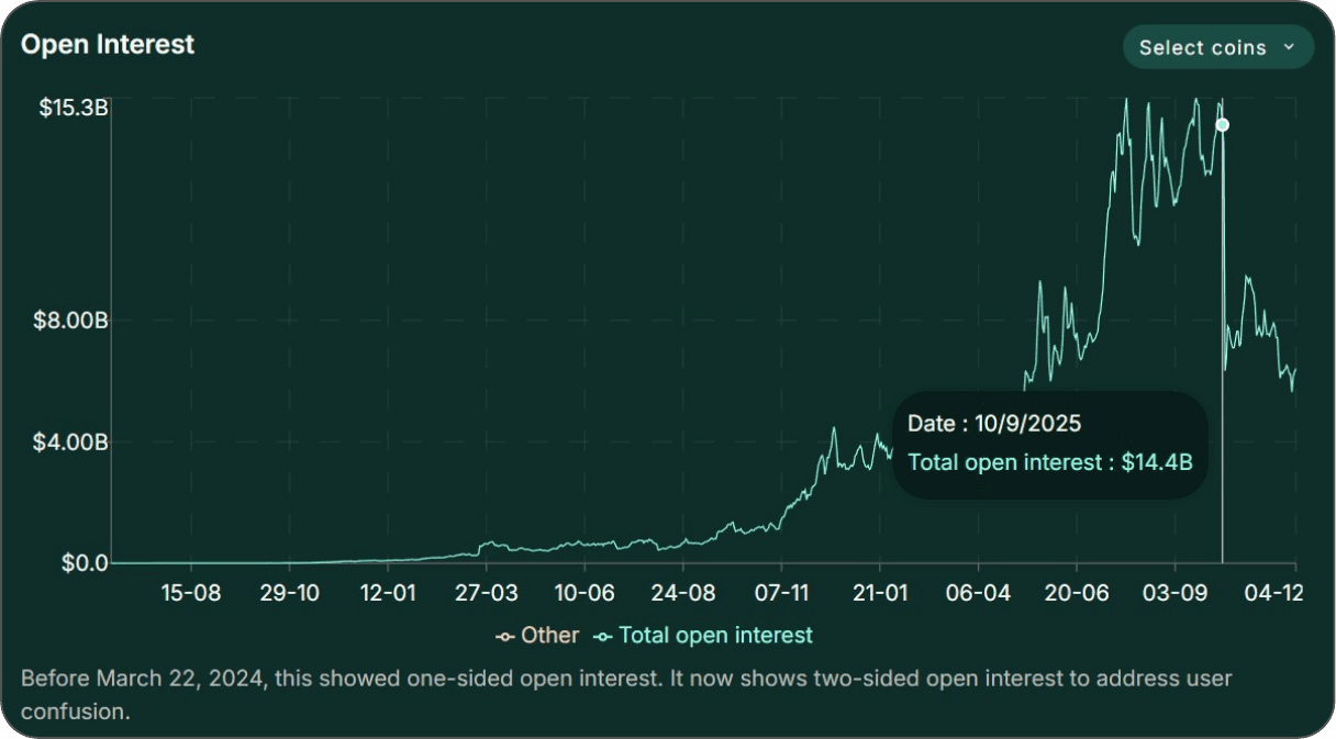
Automated execution in a thin order book exacerbates slippage.
We are addressing this via a first-principles reconstruction: maximizing liquidity access without diluting the downside capture potential.
The Large-Cap Short Inefficiency
Simply defaulting to High Market Cap tokens is not a viable hedge.
Top MC assets possess embedded structural upside drift (passive flows, flight to quality). They exhibit poor downside persistence.
Edge: None. Large caps mean-revert violently against short trend signals.
Risk: Both constrained and unconstrained models face negative expectancy (a mathematical path to zero) when forcing shorts on high-beta majors.
Optimized Universe Construction
A superior mechanics-based approach utilizes the Hyperliquid-specific universe, specifically filtering for assets eligible for 10x max leverage.
The Selection Algorithm:
Momentum Exclusion: Filter out assets displaying relative strength to avoid fighting the tape.
Liquidity Weighting: Rank the remaining universe by Open Interest (OI) to ensure execution stability.
Diversification: Select a basket of 6–10 tokens.
This structure mitigates idiosyncratic risk while isolating the specific weakness of non-major assets, balancing the need for liquidity with the necessity of volatility capture.
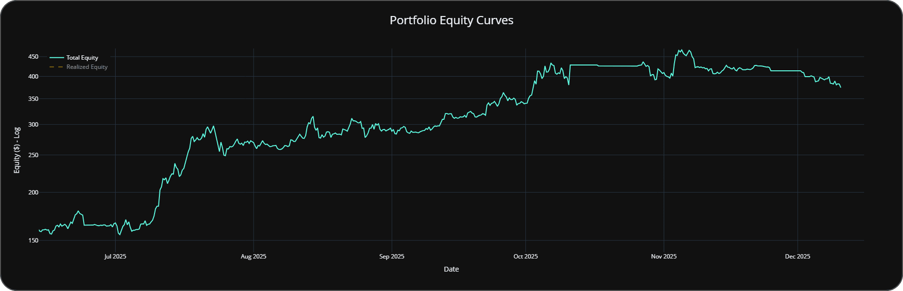
Q4 Performance Attribution
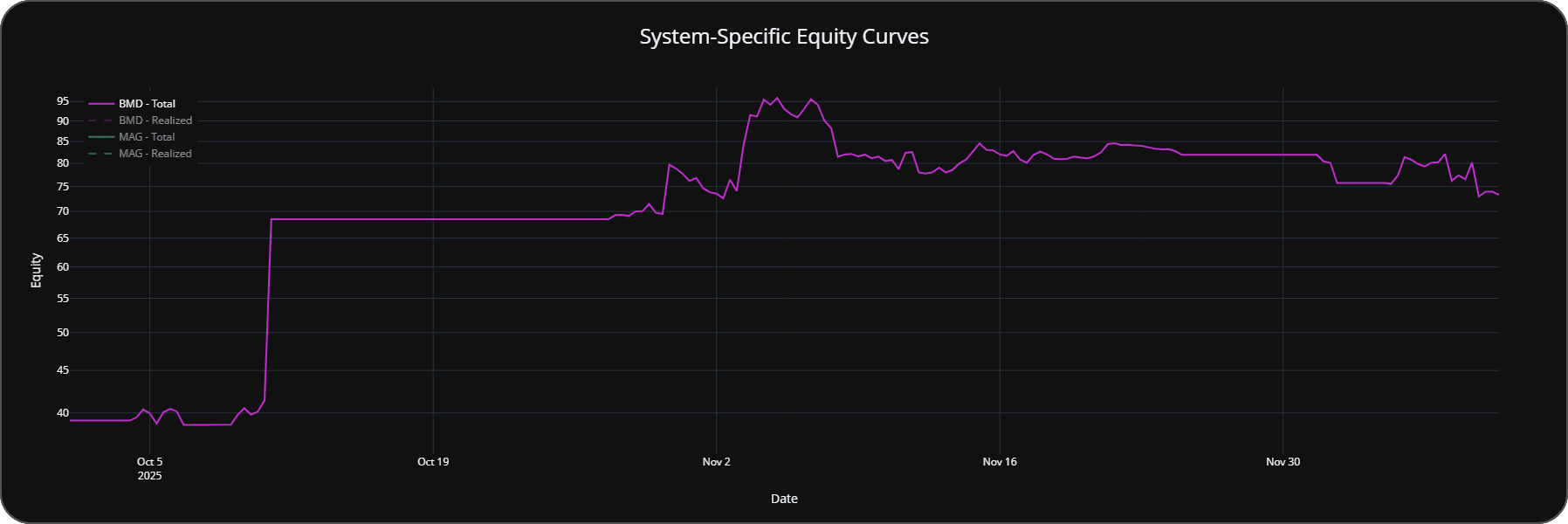
Current BMD performance reflects Q4 volatility. The primary drivers were the strategic liquidation of PENDLE (held since Oct 8th) and the high-velocity entry into ETHFI, which executed precisely at the onset of the liquidation cascade.
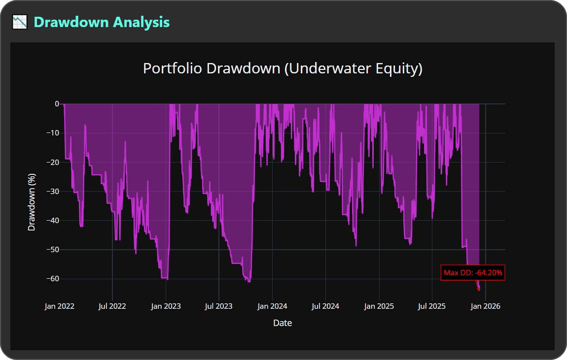
Drawdown Profile
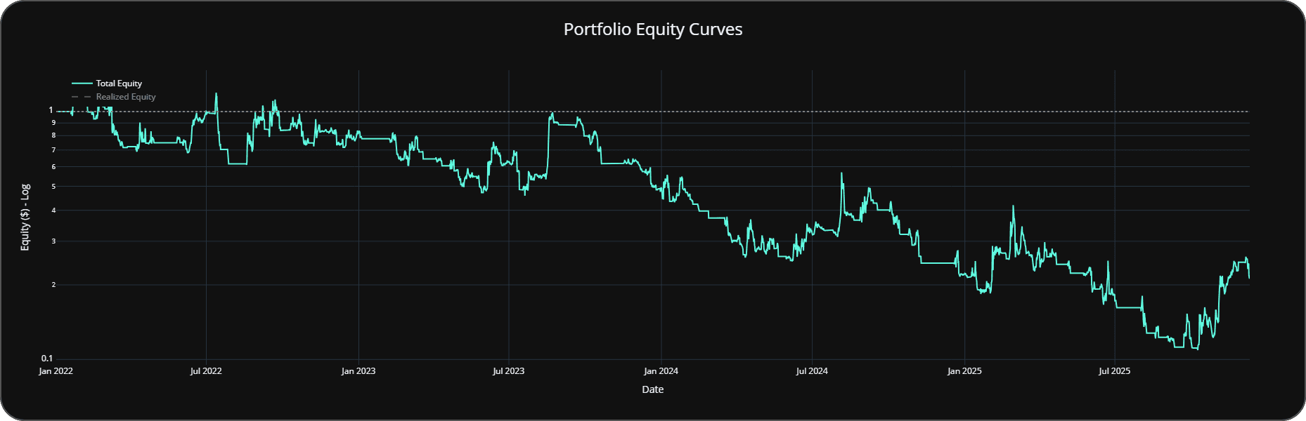
Since the allocation event, MAG has tracked the broader system weakness.
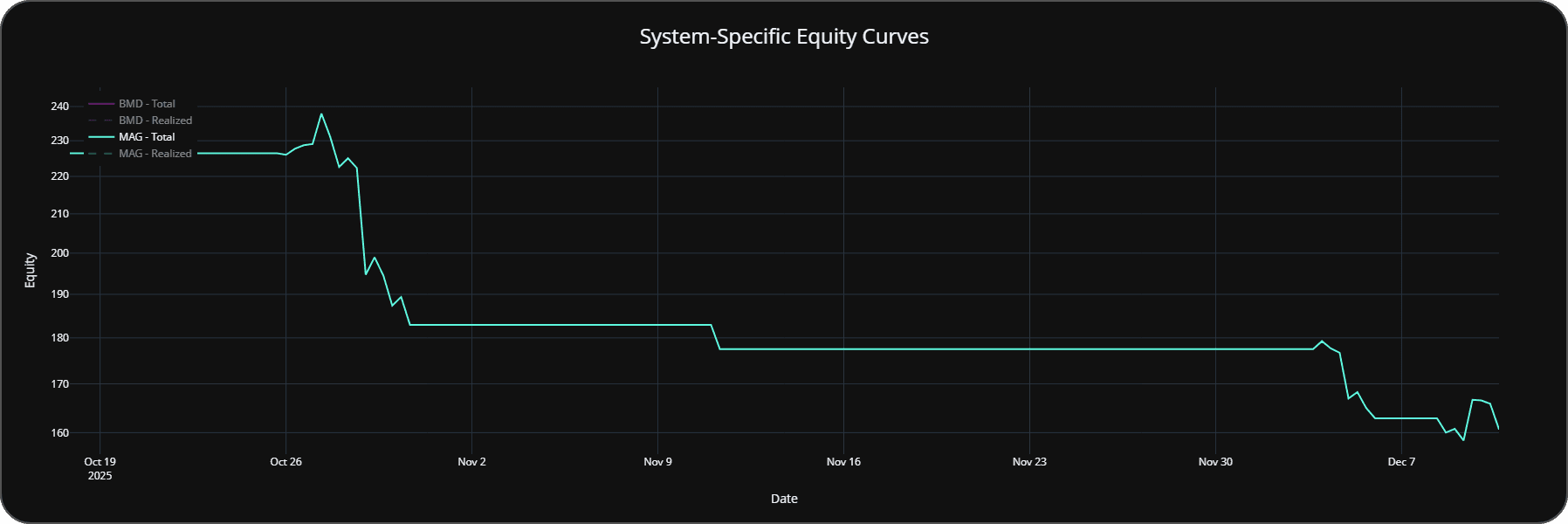
Both systems are currently experiencing a ~20% Peak-to-Trough drawdown (measured since Oct 5th). While individual account variance occurs due to execution latency, this drawdown magnitude remains strictly within the strategies risk models, return assumptions and expected variance. We do not gloss over the underperformance, but it is statistically consistent with the strategy's volatility profile.
Risk-Adjusted Metrics & Regime Analysis
Current Positioning: A review of the 60-Day Sharpe Ratio reveals a sharp compression. This metric deterioration is significant but not unprecedented within our backtested data.
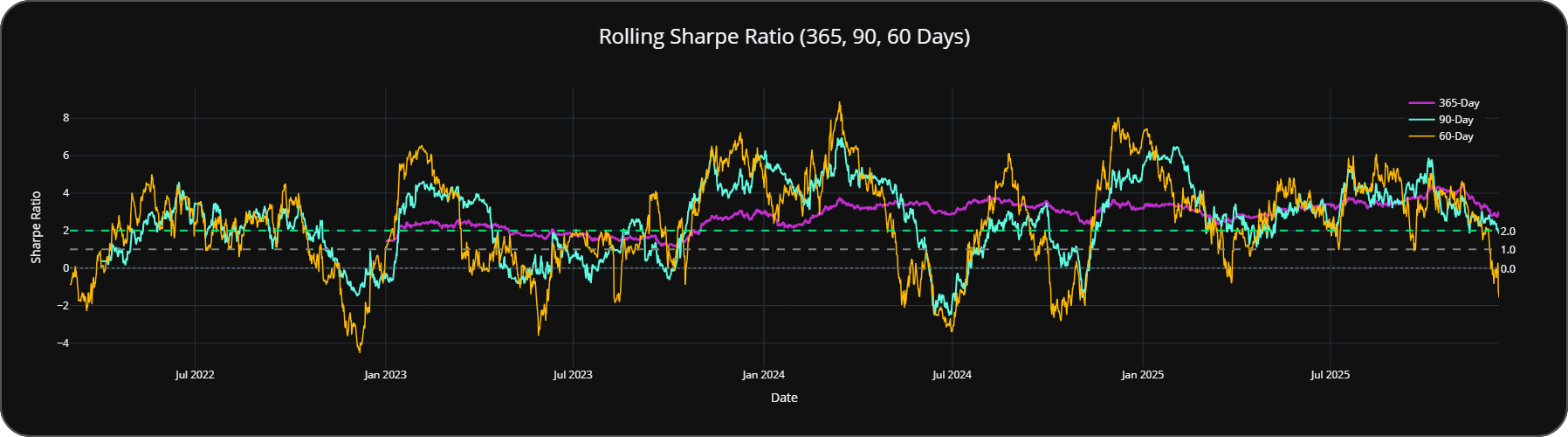
However, when isolating the individual systems, the risk-adjusted returns remain stable.


Statistical Mean Reversion
Analyzing the Rolling 7-Day Return, the portfolio currently sits at the lower bound of its statistical distribution.
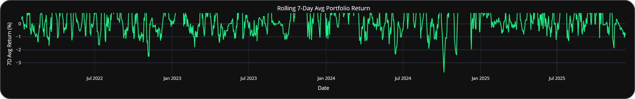
Signal: The -1% zone historically acts as a mean reversion floor.
Caveat: While probability favors a bounce, market structure does not guarantee immediate reversal.
Temporal Significance: Edge vs. Noise
As detailed in prior risk breakdowns, the Lookback Window is the critical variable in performance analysis.
90-Day Window (Quarterly): This timeframe is often insufficient for Trend strategies to realize their edge. It captures market noise and regime shifts without giving the trend component enough duration to capture fat-tail events.
365-Day Window (Annual): This timeframe provides sufficient data for high-performance outliers to normalize periods of drawdown.
The Structural Reality: Short-duration metrics (90-day) will periodically show negative Sharpe due to chop. Long-duration metrics (365-day) smooth this variance, historically maintaining a System Sharpe of ~2.5, proving that the edge is a function of time in the market, not timing the market.
Long-Only Constraints: Feasibility vs. Desirability
Is isolating the Long exposure possible? Technically, yes. Is it optimal? Emphatically, no.
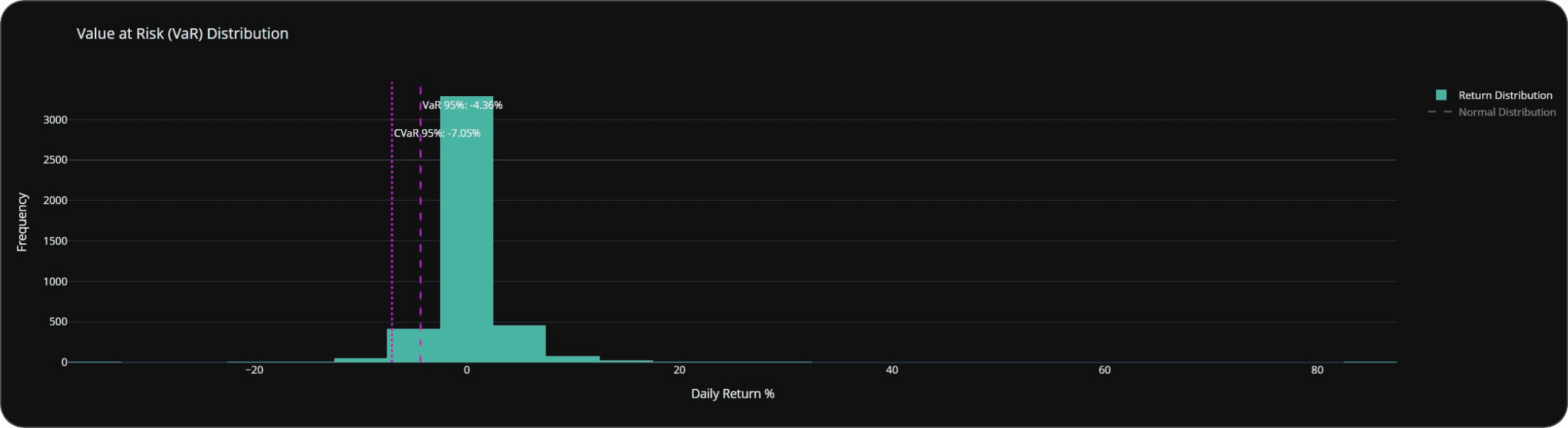
The Volatility Problem MAG operates with an annualized volatility of ~110%, characterized by extreme excess kurtosis (fat tails).
Risk Reality: Drawdowns are not linear; they are sudden and deep (~10% in single periods).
Modeling Failure: Standard risk metrics assuming a Gaussian distribution underestimate this tail risk by a magnitude of 5–10x.
MAG is engineered to chase positive convexity through trend persistence.
The Hedging Mandate
This convexity works until the left tail hits. The BMD system functions as the structural counterweight. Its mandate is to dampen the volatility inherent in "convexity-maxing."
Edge: The long side of crypto offers superior asymmetry (unbounded upside). MAG captures this effectively.
Risk: It is entirely correlation-dependent. When the market nukes, correlation goes to 1.
Current Drawdown Profile:
Regime Analysis & Liquidity Events
Since going live (June/July), the system successfully monetized the Q3 momentum before facing the Oct 10th dislocation.
The Oct 10th Liquidity Cascade This event validated the portfolio construction. The BMD component neutralized the long-side drawdown.
Mechanism: The Auto-Deleveraging (ADL) event functioned as an inadvertent optimization.
Execution Alpha: By forcing execution at the wick extremes, ADL locked in profit at maximum excursion.
Counterfactual: Without the ADL trigger, the hedge would have unwound gradually, resulting in a ~4% lower final equity capture compared to the realized spike.
Contextual Alpha & Portfolio Architecture
Analyzing performance requires more than a temporal snapshot; it demands an assessment of component interaction relative to the prevailing market regime. Building institutional-grade portfolios involves a density of context - heuristics, data granularity, and structural principles - that is often opaque to the external observer.
The "Directives" Initiative
To bridge this information gap, we are codifying our methodology into explicit Directives. These documents will serve as the architectural blueprint for a True Multi-Factor Portfolio, delineating:
Macro Structure: The high-level allocation logic.
Micro Mechanics: Specific signal generation and execution protocols.
Covariance: How distinct factors interact to dampen portfolio volatility.
Simultaneously, we are compiling a comprehensive Knowledge Base to institutionalize the strategy's intellectual capital.
Addressing Structural Vulnerabilities
Trend Following, as a single factor, possesses inherent regime fragility.
Edge: Uncapped right-tail capture during expansion.
Risk: Bleed (whipsaw) during mean-reverting chop.
We address these blind spots through automated execution of complementary signals rather than manual intervention.
The Ensemble Approach: Addition over Subtraction
The optimal response to regime-based underperformance is not to discard a valid system, but to dilute its idiosyncratic risk.
Strategy: Layer uncorrelated systems (counter-trend, mean reversion) that capture variance where Trend fails.
Objective: This additive approach smoothes the equity curve, reducing the cognitive load of drawdowns while mathematically stabilizing the compounding rate.
Overview